目录
一、PCA简介
二、数据集概览
三、数据预处理步骤
四、PCA申请
五、KMeans 聚类
六、PCA成分分析
七、逆变换
八、质心分析
九、结论
十、深入探究
10.1 第 1 步:确定 PCA 组件的最佳数量
10.2 第 2 步:使用 9 个组件重做 PCA
10.3 解释 PCA 加载和特征贡献
10.4 9项常设仲裁法院的分析与解读
10.5 如何进行主题分析
一、PCA简介
主成分分析 (PCA) 是一种统计技术,可简化高维数据的复杂性,同时保留趋势和模式。它通过将数据转换为较少的维度来实现此目的,这些维度充当特征的摘要,称为主成分 (PC)。这些分量彼此正交,确保它们表示数据中的独立方差。
二、数据集概览
在我们的案例研究中,我们使用的是 Airbnb 房源数据集,其中包含位置、房间类型、价格等各种功能。我们的目标是发现这个数据集中的潜在模式,这可以帮助我们将列表细分为有意义的组。
import pandas as pd
from sklearn.preprocessing import StandardScaler, LabelEncoder
from sklearn.decomposition import PCA
from sklearn.cluster import KMeans# Load the dataframe from the CSV file
df = pd.read_csv('https://raw.githubusercontent.com/fenago/datasets/main/airbnb.csv')
三、数据预处理步骤
在深入研究 PCA 之前,我们需要确保我们的数据是干净的,并且采用正确的分析格式:
- 缺失值:我们通过用各自列的平均值填充缺失值来处理缺失值,确保没有遗漏任何数据点。
- 分类编码:我们使用标签编码将分类变量(如 、 、 和 )转换为数字,而该特征是一次性编码的。此步骤至关重要,因为 PCA 需要数字输入。
host_is_superhostneighbourhoodproperty_typeinstant_bookablecity - 功能扩展:我们过去常常扩展功能。缩放对于 PCA 至关重要,因为它对初始变量的方差很敏感。
StandardScaler
# Fill missing values with the mean of the column
df_filled = df.fillna(df.mean())# Convert categorical columns to numeric using label encoding
# Initialize label encoder
label_encoder = LabelEncoder()# Columns to label encode
label_encode_columns = ['host_is_superhost', 'neighbourhood', 'property_type', 'instant_bookable']# Apply label encoding to each column
for column in label_encode_columns:df_filled[column] = label_encoder.fit_transform(df_filled[column])# Apply one-hot encoding to 'city' using get_dummies
df_filled = pd.get_dummies(df_filled, columns=['city'])# Redefine and refit the scaler to the current dataset
scaler = StandardScaler()
scaled_features = scaler.fit_transform(df_filled)
四、PCA申请
将 PCA 应用于我们的缩放数据集,我们决定了三个主要组成部分。这个数字通常是根据解释的方差来选择的,方差表示每个组件从数据中捕获的信息量。
# Apply PCA
pca = PCA(n_components=3)
pca_result = pca.fit_transform(scaled_features)
五、KMeans 聚类
由于我们的数据现在位于三维PCA空间中,我们应用KMeans聚类来识别四个不同的聚类。此方法对数据点进行分组,以便每个聚类中的数据点彼此之间比其他聚类中的数据点更相似。
# Apply KMeans clustering on the PCA result
kmeans_pca = KMeans(n_clusters=4, random_state=42)
kmeans_pca.fit(pca_result)
六、PCA成分分析
每个主成分都代表了原始特征的组合,但它们究竟捕获了什么?
# Get the PCA components (loadings)
pca_components = pca.components_
让我们深入研究每个 PCA 的负载:
- PC1:似乎很重视地理坐标(纬度和经度),表明该组成部分可能代表列表的地理分布。
- PC2:该组件与 host_since_datekey 负相关,表明它可能正在捕获主机经验或任期的某些方面。
- PC3:由于内住物和listing_size_sqft的负载较高,该组件可以反映列表的大小和容量。
七、逆变换
通过逆变换 PCA 聚类中心,我们将聚类映射回原始空间,以根据原始特征解释质心。这一步就像将我们的 PCA 结果翻译回我们可以理解的语言。
# Inverse transform the cluster centers from PCA space back to the original feature space
original_space_centroids = scaler.inverse_transform(pca.inverse_transform(kmeans_pca.cluster_centers_))# Create a new DataFrame for the inverse transformed cluster centers with column names
centroids_df = pd.DataFrame(original_space_centroids, columns=df_filled.columns)# Calculate the mean of the original data for comparison
original_means = df_filled.mean(axis=0)# Prepare the PCA loadings DataFrame
pca_loadings_df = pd.DataFrame(pca_components, columns=df_filled.columns, index=[f'PC{i+1}' for i in range(3)])
八、质心分析
与原始数据的平均值相比,聚类的质心告诉我们每个聚类的中心趋势。例如,如果质心的价格值高于平均值,则相应的聚类可能表示更多的优质列表。
# Append the mean of the original data to the centroids for comparison
centroids_comparison_df = centroids_df.append(original_means, ignore_index=True)# Store the PCA loadings and centroids comparison DataFrame for further analysis
pca_loadings_df.to_csv('/mnt/data/pca_loadings.csv', index=True)
centroids_comparison_df.to_csv('/mnt/data/centroids_comparison.csv', index=False)pca_loadings_df, centroids_comparison_df.head()  # Displaying the PCA loadings and the first few rows of the centroids comparison DataFrame
九、结论
PCA使我们能够降低数据集的维度,揭示最初并不明显的内在模式。当与聚类相结合时,我们可以将房源细分为不同的组,每个组代表Airbnb市场的不同方面。
十、深入探究
10.1 第 1 步:确定 PCA 组件的最佳数量
当我们执行 PCA 时,我们将原始特征集转换为一组新的正交特征,称为主成分 (PC)。每个主成分捕获数据集中总方差的一定百分比。第一个主成分捕获的方差最大,每个后续组件捕获的方差较小。通过查看累积解释方差,我们可以看到随着我们包含越来越多的分量,捕获了多少总方差。
累积解释方差图显示了通过包含最多 n 个主成分来捕获的数据集总方差的比例。这个想法是选择最少数量的主成分,这些主成分仍捕获总方差的很大一部分。一个常见的经验法则是选择足够的组件来捕获至少 95% 的总方差,这使我们能够在保留数据集中大部分信息的同时降低维度。
让我们重新审视累积解释方差图,以确定满足此条件的分量数。我们将查找累积解释方差超过 95% 的点,这通常被认为足以捕获数据集中的大部分信息。这种组件数量通常是信息保留和降维之间的良好平衡。
我们将再次分析情节并提供更直观的解释。
# Fit PCA to the data without reducing dimensions and compute the explained variance ratio
pca_full = PCA()
pca_full.fit(scaled_features)# Calculate the cumulative explained variance ratio
explained_variance_ratio = pca_full.explained_variance_ratio_
cumulative_explained_variance = explained_variance_ratio.cumsum()# Plot the cumulative explained variance ratio to find the optimal number of components
plt.figure(figsize=(10, 6))
plt.plot(range(1, len(cumulative_explained_variance) + 1), cumulative_explained_variance, marker='o', linestyle='--')
plt.title('Cumulative Explained Variance by PCA Components')
plt.xlabel('Number of PCA Components')
plt.ylabel('Cumulative Explained Variance')
plt.grid(True)
plt.axhline(y=0.95, color='r', linestyle='-')  # 95% variance line for reference
plt.text(0.5, 0.85, '95% cut-off threshold', color = 'red', fontsize=16)# Determine the number of components that explain at least 95% of the variance
optimal_num_components = len(cumulative_explained_variance[cumulative_explained_variance >= 0.95]) + 1# Highlight the optimal number of components on the plot
plt.axvline(x=optimal_num_components, color='g', linestyle='--')
plt.text(optimal_num_components + 1, 0.6, f'Optimal Components: {optimal_num_components}', color = 'green', fontsize=14)plt.show()# Returning the optimal number of components
optimal_num_components
更新后的图更清楚地说明了累积解释方差如何随着主成分数量的增加而增加。绿色垂直线标记分量数共同解释数据集中总方差的至少 95% 的点。
从图中可以看出,这个阈值有 9 个主成分。这意味着通过使用 9 个分量,我们可以捕获数据中 95% 的可变性,这通常被认为足以满足许多应用的需求。这比原始特征数量大幅减少,同时仍保留了大部分信息。
因此,在我们的分析上下文中,我们可以执行 PCA 并将维度降低到 9 个主成分,而不是使用所有原始特征,以实现更简单但仍然信息丰富的数据集表示。
10.2 第 2 步:使用 9 个组件重做 PCA
# Redo PCA with 9 components
pca_9 = PCA(n_components=9)
pca_result_9 = pca_9.fit_transform(scaled_features)# Get the PCA loadings for 9 components
pca_components_9 = pca_9.components_# Analyze the PCA loadings to determine which features contribute most to each of the 9 principal components
# We will look at the absolute values of the loadings to assess their contribution
pca_loadings_analysis_9 = pd.DataFrame(pca_components_9, columns=df_filled.columns, index=[f'PC{i+1}' for i in range(9)]
).abs().T  # Transpose to have features as rows# Sorting the loadings for each component to see the top contributing features
top_features_per_pc_9 = pca_loadings_analysis_9.apply(lambda s: s.abs().nlargest(5).index.tolist(), axis=0)top_features_per_pc_9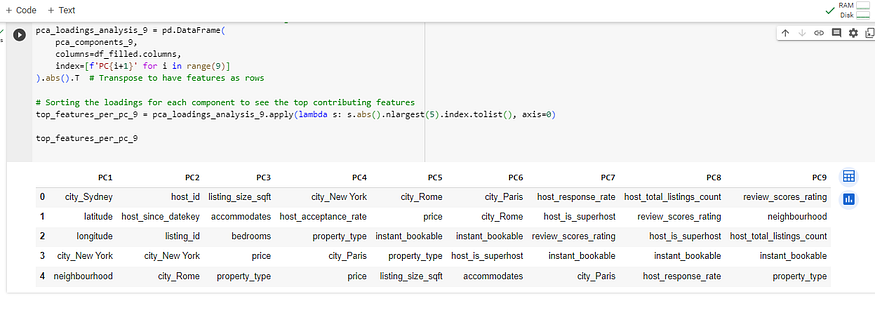
为了提供前九个主成分中每个特征的实际加载分数,我们可以输出 PCA 加载矩阵的数值。将显示给定主成分中每个特征的载荷,显示它们的贡献。
# Display the actual loadings for the top 5 features for each of the 9 principal components
# We will extract the top 5 features based on the absolute values of the loadings and display their actual loadings
import numpy as np
# Function to get top n features for each principal component with their loadings
def get_top_features_loadings(pca_loadings, n_features):top_features = {}for i in range(pca_loadings.shape[0]):# Get the index of the n largest absolute values in the i-th principal componenttop_indices = np.argsort(np.abs(pca_loadings[i]))[-n_features:]# Create a dictionary of the top features and their loadings for the i-th principal componenttop_features[f'PC{i+1}'] = {df_filled.columns[j]: pca_loadings[i][j] for j in top_indices}return top_features# Get the top 5 features and their loadings for each of the 9 principal components
top_features_loadings_9 = get_top_features_loadings(pca_components_9, 5)
top_features_loadings_9_df = pd.DataFrame(top_features_loadings_9).Ttop_features_loadings_9_df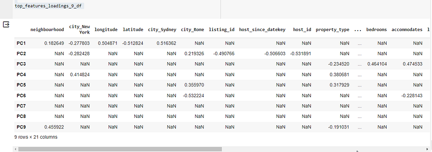
上表显示了前九个主组件中每个主组件的顶部特征的实际载荷。载荷是表示每个特征对主成分的贡献程度的系数。以下是每个主要组件的主要贡献功能及其负载的摘要:
- PC1:地理特征和城市的影响最大,载荷显示正负值,在地图上表示相反的方向。
- PC2:与主机相关的功能,如具有高负负载,这意味着这些功能与 PC2 有很强的反比关系。
host_since_datekeyhost_id - PC3:与属性相关的特征,如 、 和 具有很强的正载荷,这意味着它们直接影响 PC3。
accommodateslisting_size_sqftbedrooms - PC4 到 PC9:与城市、物业类型、预订选项和评论分数相关的各种其他功能有助于这些组件具有不同程度的正负负载。
要解释这些负载,请执行以下操作:
- 正载荷意味着随着特征值的增加,主成分的分数也会增加。
- 负载荷意味着随着特征值的增加,主成分的分数会降低。
- 载荷的大小(距零的距离)表示特征与主成分之间关系的强度。
要执行详细分析并推断每个 PCA 的含义,需要考虑数据集的领域知识,并了解每个主要功能与 Airbnb 列表的上下文之间的关系。这涉及考虑每个功能所代表的内容(例如,位置、物业大小、房东体验),以及它们如何组合在一起以形成由主组件表示的主题。
我们已经成功地对 9 个主要组件执行了 PCA,并列出了对每个组件贡献最大的前 5 个功能。以下是我们如何解释负载以确定特征贡献:
10.3 解释 PCA 加载和特征贡献
PCA 组件的载荷反映了原始变量与主成分之间的相关性。以下是解释这些负载的方法:
- 高正载荷(接近 1):表示特征与元件具有很强的正相关。
- 高负载荷(接近 -1):表示特征与元件具有很强的负关联。
- 加载接近 0:表示特征与组件的关联较弱。
每个主成分的主要贡献特征是具有最高绝对载荷的特征,无论它们是正载荷还是负载荷。这些特征被认为对组件的方差影响最大。
10.4 9项常设仲裁法院的分析与解读
现在,我们将根据主要贡献功能来解释 9 个主要组件中每个组件的主题:
- PC1:以城市相关特征和地理坐标为主,暗示了地理位置的主题。
- PC2:受房东标识符和日期的影响,表示房东经历或任期的主题。
- PC3:包括与房源面积和容量相关的功能,指向房产面积和住宿容量的主题。
- PC4:具有与城市相关的变量和接受率,暗示了托管偏好和位置可取性的主题。
- PC5:以城市和价格为标志,可能反映不同地点的定价策略主题。
- PC6:包含即时可预订和房东超赞房东状态,建议以出租服务和设施为主题。
- PC7:以回复率和评论分数为特色,指向房东响应能力和客人满意度的主题。
- PC8:还包括房东总房源和评价分数,表明房东组合和体验质量的主题。
- PC9:捕获邻域和主机列表计数,这可能表示邻域受欢迎程度和主机活动。
10.5 如何进行主题分析
要对PCA组件进行专题分析:
- 对 PCA 负载进行排序:按每个主组件的加载对特征进行排序。
- 识别主要特征:确定具有最高绝对载荷的顶级特征。
- 了解要素重要性:了解这些要素在数据集上下文中的重要性。
- 寻找模式:在顶级特征中寻找模式以推断主题。
- 考虑正负贡献:请注意,具有高正载荷的特征和具有高负载荷的特征对主题的贡献不同。
- 验证主题:使用领域知识或其他数据分析来验证推断的主题。